Regression

Notations

Goal is to find the best fitting line w0+w1*x

Evaluation

f(x) has to be as close as possible to the true value of y

Evaluation function to drive this objective

Least Squares Error = (f(x) - y) ^ 2

Objective/Loss function = J(w) = 1/2N

Optimisation

To get the best fit, the overall loss must be minimised

Done using Gradient Descent

1) Start with a initial estimate of w 2) Change w iteratively such that the loss function is minimised 3) Stop when either the minimum is hit or no improvement

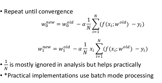
Parameter updates

Update the parameters w (weight w1 and bias w0) of the linear regressor as:

w(new) = w(old) - a * delta(J(w))

Importance of learning rate

Critical hyper-parameter to be decided by the machine learning regressor.

Too law a may lead to slower conversions Too high a may lead to oscillations

Typically a = 10^-3 is recommended for the most case

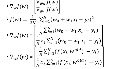
Computing Gradients

Gradient Equations

$$\frac{\partial J}{\partial w_j} = \frac{1}{N} \sum_{i=1}^{N} (f(x_i; w) - y_i)x_i^{(j)}$$

Potential Issues

• Different Scales of features
• Solution - Standardisation and Normalisation

Feature	Normalization	Standardization
Range	Fixed (usually 0 to 1)	Not fixed (usually -3 to 3)
Mean / Dev	Varies	Mean = 0, Std Dev = 1
Outliers	Very sensitive	Less sensitive
Distribution	Useful when distribution is unknown	Useful when data is Gaussian
Common Task	Image Processing, KNN	PCA, Regression, SVM