Neural Network
Neural Network Fundamentals
- Core Concept: A neural network is described as a combination of linear computation and an activation function. While traditional Machine Learning often requires manual feature extraction, Deep Learning automates this process through a "feature learning module" that learns directly from raw inputs.
- Architecture: Networks consist of multiple layers, including an input layer, hidden layers, and an output layer.
- Hidden Layers: These layers attempt to extract patterns from data. For example, in house price prediction, hidden layers might identify features like family size or school quality from raw data like the number of bedrooms or zip code.
- Propagation Equations: The process of moving through the network involves calculating $z = w \cdot x + b$ (weight multiplied by input plus bias) and then applying an activation function $a = \sigma(z)$.
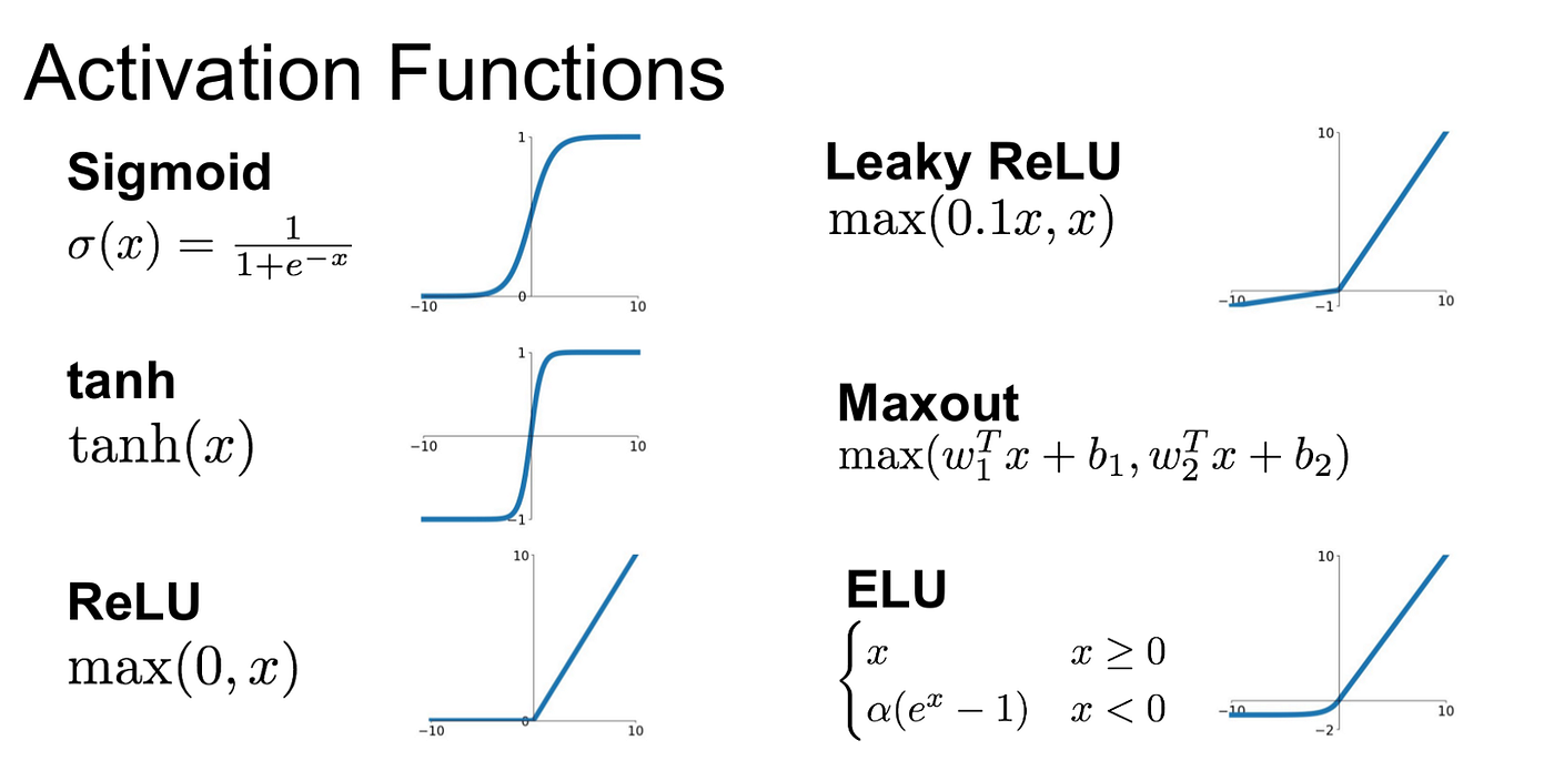
- Activation Functions: These are essential because, without them, a deep network would mathematically collapse into a simple linear regression model. Common functions mentioned include:
- Sigmoid: Used for binary classification.
- ReLU (Rectified Linear Unit): Defined as $max(0, z)$.
- Tanh: Another common non-linear activation.
- Softmax: Used in the output layer for multi-class classification to predict the probability of each class.
- Training and Optimization:
- Initialization: Weights and biases are initially set randomly. Specialized methods like Xavier Initialization and He Initialization are used to help the network converge effectively.
- Backpropagation: This is the method for updating parameters based on the loss. It utilizes a computation graph where every node represents an operation, and the chain rule is applied to calculate local and global gradients.
- Gradient Descent: The network updates its weights using the formula $w_{new} = w_{old} - \eta \frac{\partial L}{\partial w}$, where $\eta$ is the learning rate. Momentum can be added to the gradient descent process to smooth out fluctuations during learning.
- Loss Functions: For classification tasks, cross-entropy loss is frequently used.
- Improving Performance:
- Normalization: Training and testing data are often normalized to improve training stability.
- Dropout: To prevent overfitting, some neurons are randomly "dropped" during training.
- Residual/Skip Connections: These involve taking information from a previous layer and skipping one or more layers to give it to a newer layer, which helps in training deeper networks.
Convolutional Neural Networks (CNN)
CNNs are specialized neural networks designed primarily for image data, utilizing specific mathematical operations to maintain spatial relationships.
- Key Operations:
- Convolution: Instead of full connectivity, CNNs use a filter (or kernel) that slides across the input. The basic convolution formula provided is $s_t = \sum x_{t-a} w_a$.
- Padding ($P$) and Stride ($S$): These parameters control the output dimensions. Padding adds border pixels, while stride determines the step size of the filter.
- Output Dimension Formula: The width/height of the output layer ($w_2$) is calculated as: $w_2 = \frac{w_1 - F + 2P}{S} + 1$, where $F$ is the filter size.
- Flattening: Before final classification (e.g., via Softmax), the multi-dimensional feature maps are "flattened" into a one-dimensional vector.
- Unique Characteristics:
- Weight Sharing: A key feature of CNNs is that the same weights (the filter) are used across different parts of the input, reducing the total number of parameters.
- Receptive Field (RF): This refers to the specific area of the input that a particular feature in a layer "sees." It is calculated as $RF = 1 + L \times (F-1)$, where $L$ is the layer index.
- Practical Techniques:
- Data Augmentation: Creating variations of existing images (e.g., through translation or rotation) to increase the dataset size and improve robustness.
- Transfer Learning: Using a pre-trained model on a new, related task.
Broadcasting
Broadcasting is a powerful mechanism that allows you to perform mathematical operations (like addition or multiplication) between tensors of different shapes.
Activation Functions
- ReLU - The industry standard
- LeakyReLU
- Tanh - squashes values between -1 and 1
- ELU
Learning Rate
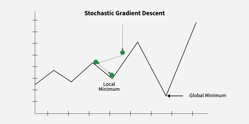
Too high - You might overshoot the minimum and model will fail to converge Too low - Training will be agonisingly slow and might get stuck in a local minimum
Optimiser
These are the algorithms that actually update the weight
SGD (Stochastic Gradient Descent) - Updates weight frequently with high noise.
Adam - It combines Momentum (keep moving in the same direction) and RMSprop (adjusting step size for each weight)
RMSprop - Introduces decay factor to prevent the learning rate from decreasing too rapidly.
| Optimizer | Advantages | Disadvantages |
|---|---|---|
| SGD | Simple, easy to implement | Slow convergence, requires tuning |
| RMSProp | Prevents fast decay of learning rates | Computationally expensive |
| Adam | Fast, combines momentum and RMSProp | Memory-intensive, computationally expensive |
| #### Training Mechanics |
Batch Size - How many samples the model looks at before updating weights - Small - More noise, but better generalisation
Number of Epochs - How many full passes the model makes through the entire dataset
Initialisation and Regularisation
Weight Initialisation - Starting weights at exactly causes same updates. We can use He initialisation (For ReLU) and Xavier (for Tanh and Sigmoid) to keep variance steady across layers
Dropout - Randomly turn off a percentage of neurons during training. This forces the network to depend overly on unwanted neurons.
The derivation for the backpropagation of the Softmax activation function with Cross-Entropy loss is centered on finding $\frac{\partial L}{\partial z_i}$. This is divided into two main parts: the derivative of the Softmax function and the derivative of the Loss function.
1. The Softmax Function and Loss Function
The Softmax activation for the $i$-th neuron in the output layer is defined as:
$$a_i = \frac{e^{z_i}}{\sum_{k=1}^{n} e^{z_k}}$$
The Cross-Entropy loss for a single observation is:
$$L = -\sum_{k=1}^{n} y_k \ln(a_k)$$
2. Derivative of Softmax: $\frac{\partial a_i}{\partial z_j}$
There are two cases when differentiating $a_i$ with respect to $z_j$:
Case 1: When $i = j$
Using the quotient rule $\left(\frac{u}{v}\right)' = \frac{v u' - u v'}{v^2}$:
$$\frac{\partial a_i}{\partial z_i} = \frac{(\sum e^{z_k})e^{z_i} - e^{z_i}(e^{z_i})}{(\sum e^{z_k})^2}$$
$$\frac{\partial a_i}{\partial z_i} = \frac{e^{z_i}}{\sum e^{z_k}} \cdot \frac{\sum e^{z_k} - e^{z_i}}{\sum e^{z_k}} = a_i(1 - a_i)$$
Case 2: When $i \neq j$
$$\frac{\partial a_i}{\partial z_j} = \frac{(\sum e^{z_k})(0) - e^{z_i}(e^{z_j})}{(\sum e^{z_k})^2}$$
$$\frac{\partial a_i}{\partial z_j} = -\frac{e^{z_i}}{\sum e^{z_k}} \cdot \frac{e^{z_j}}{\sum e^{z_k}} = -a_i a_j$$
3. Derivative of Loss with respect to $z_i$
We apply the chain rule: $\frac{\partial L}{\partial z_i} = \sum_{k=1}^{n} \frac{\partial L}{\partial a_k} \frac{\partial a_k}{\partial z_i}$.
Substituting $\frac{\partial L}{\partial a_k} = -\frac{y_k}{a_k}$:
$$\frac{\partial L}{\partial z_i} = -\frac{y_i}{a_i} \cdot \frac{\partial a_i}{\partial z_i} + \sum_{k \neq i} \left( -\frac{y_k}{a_k} \cdot \frac{\partial a_k}{\partial z_i} \right)$$
Substitute the Softmax derivatives from Step 2:
$$\frac{\partial L}{\partial z_i} = -\frac{y_i}{a_i} \cdot a_i(1 - a_i) + \sum_{k \neq i} \left( -\frac{y_k}{a_k} \cdot (-a_k a_i) \right)$$
$$\frac{\partial L}{\partial z_i} = -y_i(1 - a_i) + \sum_{k \neq i} y_k a_i$$
$$\frac{\partial L}{\partial z_i} = -y_i + y_i a_i + \sum_{k \neq i} y_k a_i$$
Factoring out $a_i$:
$$\frac{\partial L}{\partial z_i} = a_i \left( y_i + \sum_{k \neq i} y_k \right) - y_i$$
$$\frac{\partial L}{\partial z_i} = a_i \left( \sum_{k=1}^{n} y_k \right) - y_i$$
Since $y$ is a one-hot encoded vector, $\sum y_k = 1$:
$$\frac{\partial L}{\partial z_i} = a_i - y_i$$
Final Result
In vector form for the output layer (layer 3 in the video's notation):
$$dz^{[3]} = a^{[3]} - y$$
This elegant result shows that the gradient for multi-class classification using Softmax and Cross-Entropy is simply the difference between the predicted probabilities and the actual ground truth, matching the result found in binary classification with Sigmoid.